The Travelling Salesman Problem: 4 Exact Methods Explained

Introduction

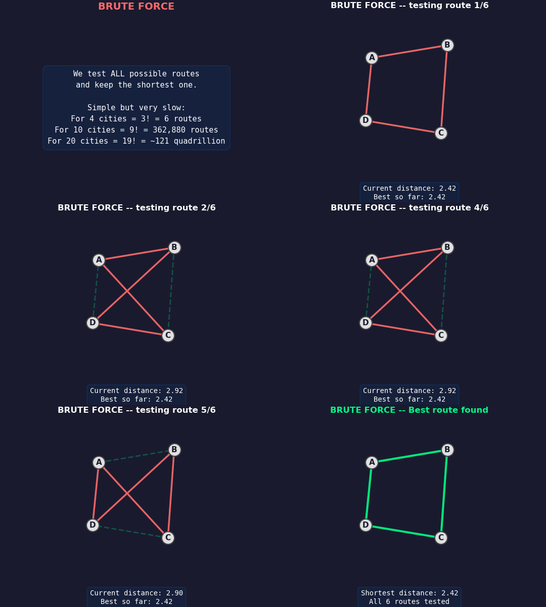
The Travelling Salesman Problem (TSP) is a classic in computer science and operations research:

Given a set of cities and the distances between each pair, what's the shortest route that visits every city exactly once and returns to the starting point?

Despite how simple it sounds, TSP is NP-hard — there's no known polynomial-time algorithm that works on all instances. That's why it's become the go-to benchmark for testing optimization techniques.

In this article, we walk through four exact methods (which guarantee the optimal solution) with visual animations for each.

1. Brute Force — Exhaustive Enumeration

Brute Force Animation

Idea

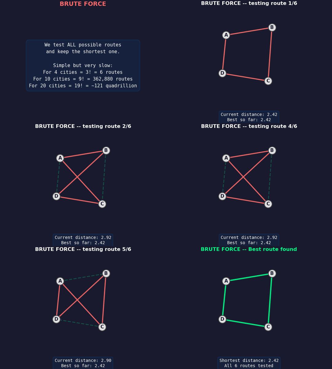
The simplest way: enumerate every permutation of the cities, compute the cost of each tour, and keep the best one.

Complexity

\text{Number of tours} = (n-1)! \quad \Rightarrow \quad O(n!)

For $n = 10$ cities that's $362\,880$ tours — manageable. For $n = 20$ it's $\approx 1.2 \times 10^{17}$ — completely infeasible.

Code

python

def brute_force_tsp(distances, n):
    cities = list(range(1, n))  # fix city 0 as the starting point
    best_cost = float('inf')
    best_tour = None

    for perm in permutations(cities):
        tour = [0] + list(perm) + [0]
        cost = sum(distances[tour[i]][tour[i+1]] for i in range(n))
        if cost < best_cost:
            best_cost = cost
            best_tour = tour

    return best_tour, best_cost

When to use it?

Very small number of cities ( $n \leq 12$ )
As a reference to validate other algorithms

2. Dynamic Programming — The Held-Karp Algorithm

Dynamic Programming Animation

Idea

The Held-Karp algorithm (1962) uses memoization to avoid recomputing the same sub-problems. Each state is a pair $(S, j)$ :

$S$ — the set of cities already visited (encoded as a bitmask)
$j$ — the last city visited

The recurrence relation:

C(S, j) = \min_{i \in S \setminus \{j\}} \left[ C(S \setminus \{j\}, i) + d(i, j) \right]

Complexity

O(n^2 \cdot 2^n)

This is exponentially better than $O(n!)$ . For $n = 20$ , we go from $10^{17}$ down to $\approx 4 \times 10^8$ operations — solvable in seconds.

Code

python

def held_karp(distances, n):
    # dp[(S, j)] = min cost to visit the cities in S, ending at j
    dp = {}
    # Base case: start from city 0
    for j in range(1, n):
        dp[(1 << j, j)] = distances[0][j]

    for size in range(2, n):
        for S in combinations(range(1, n), size):
            bits = sum(1 << v for v in S)
            for j in S:
                bits_without_j = bits & ~(1 << j)
                dp[(bits, j)] = min(
                    dp[(bits_without_j, i)] + distances[i][j]
                    for i in S if i != j
                )

    # Close the cycle: return to city 0
    all_bits = (1 << n) - 2  # all cities except 0
    return min(dp[(all_bits, j)] + distances[j][0] for j in range(1, n))

Advantages

Much faster than brute force
Guarantees the optimal solution
Practical for up to $n \approx 25$ cities

3. Branch and Bound — Smart Pruning

Branch and Bound Animation

Idea

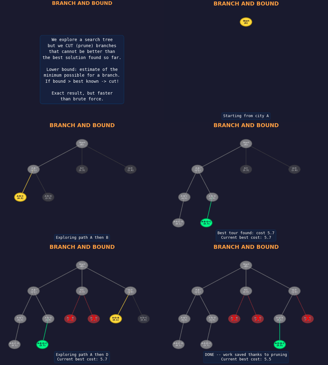
Branch and Bound explores a search tree by building tours city by city. At each node, a lower bound on the best achievable solution is computed. If this bound exceeds the best known solution, the branch is pruned (cut off).

Key steps:

Branch: choose the next city to visit
Bound: calculate a lower bound (often via a relaxation, e.g. MST)
Prune: discard unpromising branches

Typical lower bound

A common choice is the Minimum Spanning Tree (MST) of the unvisited cities:

\text{bound} = \text{partial cost} + \text{MST of remaining cities}

Code

python

def branch_and_bound_tsp(distances, n):
    best_cost = float('inf')
    best_tour = None

    def explore(tour, cost, visited):
        nonlocal best_cost, best_tour

        if len(tour) == n:
            total_cost = cost + distances[tour[-1]][tour[0]]
            if total_cost < best_cost:
                best_cost = total_cost
                best_tour = tour[:]
            return

        for city in range(n):
            if city not in visited:
                new_cost = cost + distances[tour[-1]][city]
                bound = new_cost + mst_bound(distances, visited | {city}, n)
                if bound < best_cost:  # prune if unpromising
                    tour.append(city)
                    visited.add(city)
                    explore(tour, new_cost, visited)
                    tour.pop()
                    visited.remove(city)

    explore([0], 0, {0})
    return best_tour, best_cost

Performance

In practice, Branch and Bound can solve instances of 30 to 40 cities (and sometimes more with good bounding heuristics). The quality of the lower bound is critical.

4. Integer Linear Programming (ILP)

ILP Animation

Idea

We formulate the TSP as an Integer Linear Program (ILP). Binary variables $x_{ij} \in \{0, 1\}$ indicate whether edge $(i, j)$ is part of the tour.

Formulation

\min \sum_{i} \sum_{j \neq i} d_{ij} \cdot x_{ij}

Subject to:

Each city is left exactly once: $\sum_{j \neq i} x_{ij} = 1 \quad \forall i$
Each city is entered exactly once: $\sum_{i \neq j} x_{ij} = 1 \quad \forall j$
Sub-tour elimination (Miller-Tucker-Zemlin constraints): $u_i - u_j + n \cdot x_{ij} \leq n - 1 \quad \forall i, j \geq 1$

Implementation with a solver

python

from ortools.linear_solver import pywraplp

def ilp_tsp(distances, n):
    solver = pywraplp.Solver.CreateSolver('SCIP')

    # Binary decision variables
    x = {}
    for i in range(n):
        for j in range(n):
            if i != j:
                x[i, j] = solver.BoolVar(f'x_{i}_{j}')

    # Objective: minimize total distance
    solver.Minimize(
        sum(distances[i][j] * x[i, j]
            for i in range(n) for j in range(n) if i != j)
    )

    # Constraints: leave and enter each city exactly once
    for i in range(n):
        solver.Add(sum(x[i, j] for j in range(n) if j != i) == 1)
        solver.Add(sum(x[j, i] for j in range(n) if j != i) == 1)

    # Sub-tour elimination (MTZ)
    u = [solver.IntVar(0, n - 1, f'u_{i}') for i in range(n)]
    for i in range(1, n):
        for j in range(1, n):
            if i != j:
                solver.Add(u[i] - u[j] + n * x[i, j] <= n - 1)

    solver.Solve()
    return extract_tour(x, n)

Advantages

Leverages industrial-grade solvers (Gurobi, CPLEX, SCIP)
Can handle instances of hundreds of cities with the right techniques (cuts, LP relaxation)
Very flexible — easy to add extra constraints

Comparison

Method	Complexity	Max cities (practical)	Optimal guarantee
Brute Force	$O(n!)$	~12	Yes
Held-Karp (DP)	$O(n^2 \cdot 2^n)$	~25	Yes
Branch & Bound	Variable	~40	Yes
ILP (solver)	Variable	~100+	Yes

Wrapping Up

TSP is a perfect example of how a simple question can hide massive computational complexity. All four methods here guarantee the optimal solution, but they differ dramatically in efficiency:

Brute force is educational but unusable beyond 12 cities
Dynamic programming (Held-Karp) is the first real algorithmic speedup
Branch and Bound adds intelligence to the search
Integer Linear Programming harnesses the power of modern solvers

For large-scale instances (thousands of cities), we turn to approximate methods — greedy algorithms, 2-opt, simulated annealing, genetic algorithms, ant colony optimization. But that's a topic for another post.

Questions or suggestions? Hit me up via the contact page.

The Travelling Salesman Problem: 4 Exact Methods Explained

Introduction

1. Brute Force — Exhaustive Enumeration

Idea

Complexity

Code

When to use it?

2. Dynamic Programming — The Held-Karp Algorithm

Idea

Complexity

Code

Advantages

3. Branch and Bound — Smart Pruning

Idea

Typical lower bound

Code

Performance

4. Integer Linear Programming (ILP)

Idea

Formulation

Implementation with a solver

Advantages

Comparison

Wrapping Up

Comments

Get notified of new posts